Instructions For linux (Very similar for MACOS)
One time installations
Open a Command Prompt (cmd) window (ctrl+T) and type the
following:
python -m pip install –-upgrade pip
python -m pip install –-upgrade setuptools
python -m pip install wheel
After that you can install the planet-hunting scientific programs
entering these lines:
python -m pip install lightkurve
Now you are ready to search for exoplanets!
Light Curve Analysis
Create a “.py” file in which you will insert the bold lines
shown below. After that you open the terminal and visit the directory
of the file you created. You run the python code using the python3
command (for example: python3 exampleFile.py).
import lightkurve as lk
import matplotlib.pyplot as plt
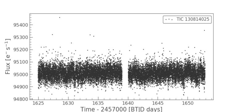
Now, let’s see one example. Say that you want to download the
light curve of TIC 130814025, a star observed by the TESS Space
Telescope. Type:
lc = lk.search_lightcurve("TIC130814025").download()Now you have downloaded your first light curve from TESS!!
If you want to see your amazing light curve, type:
lc.scatter()
plt.show()
If there are more than one data files (that is, there are
observations from more than one sectors) then you use the
download_all() command:
lc =lk.search_lightcurve("TIC130814025").download_all()lc1=lc.stitch()
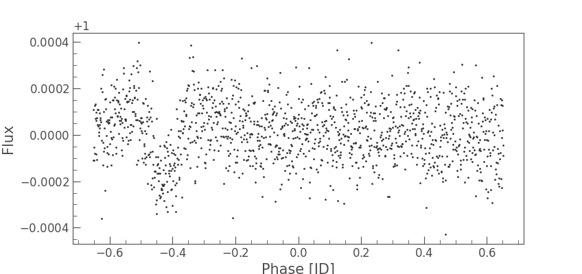
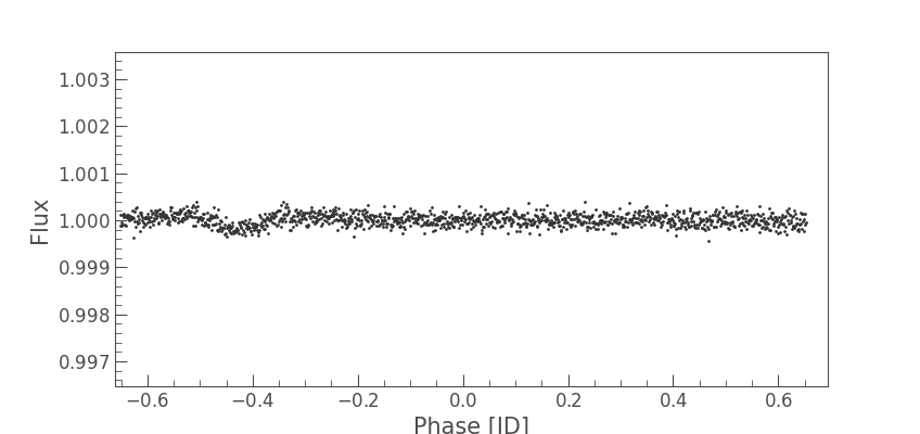
Then you continue as follows:
lc2=lc.remove_nans().remove_outliers().normalize().flatten(window_length=401)
OR in case you have more than one files
lc2=lc1.remove_nans().remove_outliers().normalize().flatten(window_length=401)
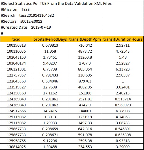
lc2.to_csv('C:\tessfiles\lc2.csv')   #You can use this command to save the folded lightcurve to a csv
file for further analysis with pltrack1 or other programs
# You should also change the C:\tessfiles to your preferred path
planet=lc2.fold(period=1.30488).bin(time_bin_size=0.001)
planet.scatter()
plt.show()
The type of the graphs expected are like the ones shown
above.